In the ever-evolving landscape of machine learning, binary classification stands as a cornerstone technique, powering countless applications that shape our digital world. From the seemingly simple task of filtering spam emails to the life-saving potential of early disease detection, binary classification algorithms are the unsung heroes working behind the scenes. This comprehensive guide will take you on a journey through the intricacies of binary classification, with a special focus on activation functions, loss calculations, and a hands-on PyTorch implementation.
The Fundamentals of Binary Classification
At its core, binary classification is the task of categorizing input data into one of two possible classes. It's the digital equivalent of sorting items into two distinct piles, each representing a specific category or outcome. This fundamental concept forms the basis for more complex machine learning problems and is essential for any aspiring data scientist or AI engineer to master.
The Ubiquity of Binary Classification
The applications of binary classification are vast and varied, touching nearly every aspect of our digital lives:
In the realm of cybersecurity, binary classifiers act as vigilant gatekeepers, distinguishing between benign and malicious network traffic. Financial institutions rely on these algorithms to detect fraudulent transactions, safeguarding millions of accounts worldwide. In healthcare, binary classification models assist in diagnosing diseases, potentially saving lives through early detection. E-commerce platforms use these techniques to predict customer behavior, enhancing user experiences and driving sales.
The power of binary classification lies in its simplicity and versatility. By understanding this fundamental concept, you unlock the potential to solve a myriad of real-world problems across diverse industries.
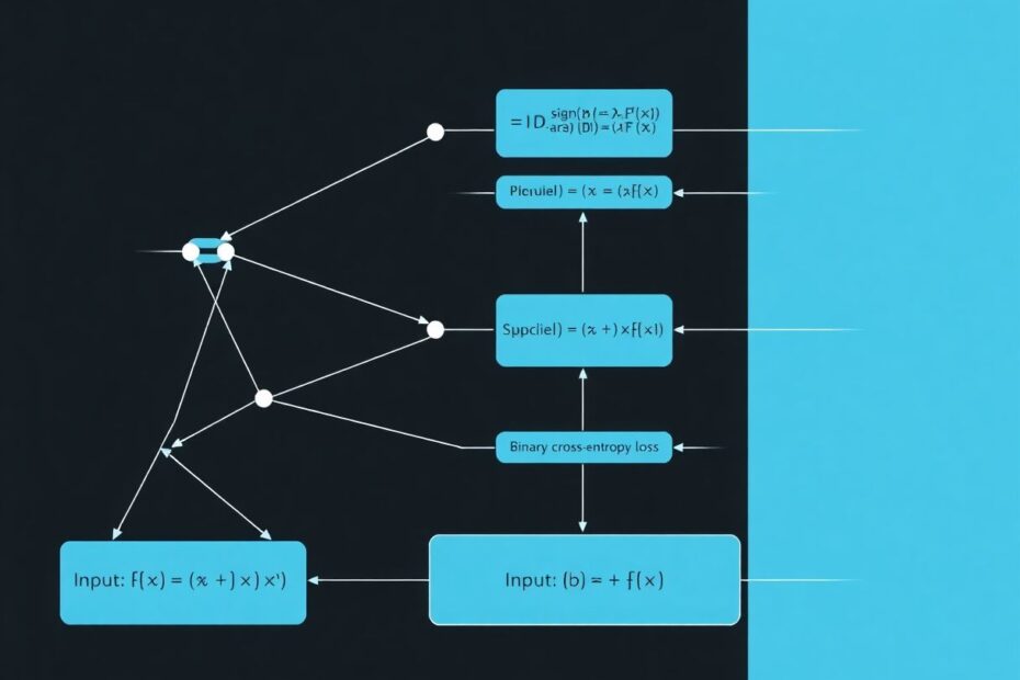
The Architecture of a Binary Classifier
To truly grasp binary classification, we must dissect the anatomy of a typical model. A binary classifier consists of several key components working in harmony:
The Input Layer: This is where our journey begins. The input layer receives the raw features of our data, acting as the sensory organs of our model. These features could be pixel values of an image, word frequencies in a text, or any other relevant attributes of the data we're trying to classify.
Hidden Layers: The hidden layers are where the magic happens. These layers process and transform the input data, learning increasingly complex representations as we go deeper into the network. The number and size of these hidden layers can vary, allowing for different levels of model complexity.
The Output Layer: At the end of our neural journey, we arrive at the output layer. For binary classification, this layer typically consists of a single neuron, whose activation represents the model's prediction.
Activation Function: The activation function is the heartbeat of our classifier. It transforms the raw output of the neuron into a probability, allowing us to interpret the model's prediction. For binary classification, the sigmoid function reigns supreme.
Loss Function: The loss function serves as our model's compass, guiding it towards better predictions. It quantifies how far off our predictions are from the true labels, providing a signal for the model to learn and improve.
The Sigmoid Activation Function: The Probability Transformer
The sigmoid function is the unsung hero of binary classification, playing a crucial role in transforming our model's raw output into a meaningful probability. Let's dive deeper into this mathematical marvel.
The Mathematics Behind Sigmoid
The sigmoid function, denoted as σ(x), is defined by the following equation:
σ(x) = 1 / (1 + e^(-x))
Where 'e' is the base of natural logarithms (approximately 2.71828) and 'x' is the input value.
This elegant function has several properties that make it ideal for binary classification:
Output Range: The sigmoid function always produces values between 0 and 1, perfectly aligning with our need to represent probabilities.
Smooth Gradient: The function has a smooth, differentiable curve, which is crucial for efficient backpropagation during the training process.
Non-linearity: By introducing non-linearity into our network, the sigmoid function allows our model to learn complex, non-linear decision boundaries.
Implementing Sigmoid in PyTorch
While PyTorch provides a built-in sigmoid function, understanding its implementation can deepen our appreciation for this crucial component. Here's how we can implement the sigmoid function from scratch:
import torch

def custom_sigmoid(x):
    return 1 / (1 + torch.exp(-x))

# Example usage
input_tensor = torch.randn(5)
output = custom_sigmoid(input_tensor)
print(f"Input: {input_tensor}")
print(f"Sigmoid Output: {output}")
This implementation showcases the simplicity and elegance of the sigmoid function. By applying this function to our model's output, we transform raw scores into interpretable probabilities, laying the foundation for our binary classification decisions.
Binary Cross-Entropy Loss: The Learning Signal
Once our model produces a prediction, we need a way to quantify its performance. Enter the Binary Cross-Entropy (BCE) loss function, the guiding light that helps our model learn and improve.
The Mathematics of BCE Loss
The BCE loss function is defined as:
BCE = -[y * log(p) + (1 - y) * log(1 - p)]
Where:
- y is the true label (0 or 1)
- p is the predicted probability
This formula might look intimidating at first glance, but it encapsulates a profound concept. Let's break it down:
- When the true label is 1 (y = 1), the loss is primarily determined by -log(p). This term heavily penalizes the model when it predicts a low probability for a positive example.
- When the true label is 0 (y = 0), the loss is governed by -log(1 – p). This term penalizes the model for assigning high probabilities to negative examples.
The Brilliance of BCE Loss
The BCE loss function is more than just a mathematical formula; it's a carefully designed learning signal with several key advantages:
Penalizes Confident Mistakes: BCE loss doesn't just care about whether the prediction is right or wrong; it cares about how confident the model is in its prediction. A model that is very confident in a wrong prediction will incur a much higher loss than one that is less certain.
Encourages Certainty: On the flip side, BCE loss rewards the model for being more certain about correct predictions. This encourages the model to make clear, decisive predictions when it has strong evidence.
Mathematically Sound: BCE loss is derived from principles of information theory and maximum likelihood estimation. This solid theoretical foundation ensures that minimizing BCE loss leads to optimal probability estimates.
Implementing BCE Loss in PyTorch
While PyTorch provides a built-in BCE loss function, implementing it ourselves can provide valuable insights:
import torch

def custom_bce_loss(predictions, targets):
    epsilon = 1e-15  # Small value to avoid log(0)
    predictions = torch.clamp(predictions, min=epsilon, max=1 - epsilon)
    loss = -torch.mean(targets * torch.log(predictions) + (1 - targets) * torch.log(1 - predictions))
    return loss

# Example usage
predictions = torch.tensor([0.7, 0.3, 0.9])
targets = torch.tensor([1.0, 0.0, 1.0])
loss = custom_bce_loss(predictions, targets)
print(f"BCE Loss: {loss.item()}")
This implementation includes a small epsilon value to prevent numerical instability when taking logarithms of very small numbers. The torch.clamp function ensures our predictions stay within a valid probability range.
A Complete PyTorch Binary Classification Model
Now that we've explored the key components, let's bring everything together in a complete PyTorch binary classification model. This example will showcase how activation functions and loss calculations come together in a practical implementation.
import torch
import torch.nn as nn
import torch.optim as optim
from torch.utils.data import DataLoader, TensorDataset
from sklearn.datasets import make_classification
from sklearn.model_selection import train_test_split
from sklearn.metrics import roc_auc_score

# Generate synthetic data
X, y = make_classification(n_samples=1000, n_features=20, n_classes=2, random_state=42)
X_train, X_test, y_train, y_test = train_test_split(X, y, test_size=0.2, random_state=42)

# Convert to PyTorch tensors
X_train = torch.FloatTensor(X_train)
y_train = torch.FloatTensor(y_train)
X_test = torch.FloatTensor(X_test)
y_test = torch.FloatTensor(y_test)

# Create DataLoader
train_dataset = TensorDataset(X_train, y_train)
train_loader = DataLoader(train_dataset, batch_size=32, shuffle=True)

# Define the model
class BinaryClassifier(nn.Module):
    def __init__(self, input_size):
        super(BinaryClassifier, self).__init__()
        self.layer1 = nn.Linear(input_size, 64)
        self.layer2 = nn.Linear(64, 32)
        self.layer3 = nn.Linear(32, 1)

    def forward(self, x):
        x = torch.relu(self.layer1(x))
        x = torch.relu(self.layer2(x))
        x = torch.sigmoid(self.layer3(x))
        return x

# Initialize model, loss, and optimizer
model = BinaryClassifier(input_size=20)
criterion = nn.BCELoss()
optimizer = optim.Adam(model.parameters(), lr=0.001)

# Training loop
def train_model(model, train_loader, criterion, optimizer, epochs=100):
    model.train()
    for epoch in range(epochs):
        for batch_idx, (data, target) in enumerate(train_loader):
            optimizer.zero_grad()
            output = model(data)
            loss = criterion(output, target.unsqueeze(1))
            loss.backward()
            optimizer.step()

        if (epoch + 1) % 10 == 0:
            print(f'Epoch {epoch+1}/{epochs}, Loss: {loss.item():.4f}')

# Train the model
train_model(model, train_loader, criterion, optimizer)

# Evaluation
def evaluate_model(model, X_test, y_test):
    model.eval()
    with torch.no_grad():
        outputs = model(X_test)
        predicted = (outputs > 0.5).float()
        accuracy = (predicted.squeeze() == y_test).float().mean()
        auc_roc = roc_auc_score(y_test, outputs)

    print(f'Accuracy: {accuracy.item():.4f}')
    print(f'AUC-ROC: {auc_roc:.4f}')

# Evaluate the model
evaluate_model(model, X_test, y_test)
This comprehensive example demonstrates how to:
- Generate synthetic data for binary classification
- Create a custom PyTorch model with sigmoid activation in the output layer
- Implement a training loop using Binary Cross-Entropy loss
- Evaluate the model's performance using accuracy and AUC-ROC metrics
By running this code, you'll see the model's loss decrease over time and get a final evaluation of its performance on the test set.
Advanced Considerations in Binary Classification
While we've covered the core concepts, the world of binary classification is rich with advanced techniques and considerations:
Handling Imbalanced Datasets
In many real-world scenarios, one class may be significantly underrepresented in the dataset. This class imbalance can lead to models that perform poorly on the minority class. Techniques to address this include:
- Oversampling the minority class (e.g., SMOTE – Synthetic Minority Over-sampling Technique)
- Undersampling the majority class
- Using weighted loss functions to give more importance to the minority class
Feature Engineering and Selection
The quality of your input features can dramatically impact model performance. Advanced techniques in this area include:
- Principal Component Analysis (PCA) for dimensionality reduction
- Recursive Feature Elimination (RFE) to identify the most important features
- Creating interaction terms between existing features
Ensemble Methods
Combining multiple models can often lead to better performance than any single model. Popular ensemble methods for binary classification include:
- Random Forests: Combining multiple decision trees
- Gradient Boosting Machines (e.g., XGBoost, LightGBM)
- Stacking: Using predictions from multiple models as inputs to a meta-model
Hyperparameter Tuning
Finding the optimal set of hyperparameters can significantly boost model performance. Advanced techniques include:
- Grid Search: Exhaustively searching through a predefined set of hyperparameters
- Random Search: Randomly sampling from a distribution of hyperparameters
- Bayesian Optimization: Using probabilistic models to guide the search for optimal hyperparameters
Model Interpretability
As binary classifiers are often used in critical decision-making processes, understanding why a model makes certain predictions is crucial. Techniques for model interpretability include:
- SHAP (SHapley Additive exPlanations) values
- LIME (Local Interpretable Model-agnostic Explanations)
- Feature importance analysis
Conclusion: The Journey of Binary Classification
As we conclude our deep dive into binary classification, it's clear that this fundamental technique is far more than a simple yes-or-no decision maker. It's a powerful tool that forms the bedrock of many complex machine learning systems, driving innovations across industries and improving our daily lives in countless ways.
From the elegant mathematics of the sigmoid function to the learning signal provided by Binary Cross-Entropy loss, we've explored the key components that make binary classification tick. Our PyTorch implementation brings these concepts to life, demonstrating how theory translates into practical, working code.
But remember, this is just the beginning of your journey. The field of machine learning is vast and ever-evolving, with new techniques and applications emerging constantly. As you continue to explore and experiment, keep pushing the boundaries of what's possible with binary classification.
Whether you're building the next breakthrough in medical diagnosis, enhancing cybersecurity systems, or pioneering new frontiers in AI, the principles we've discussed here will serve as your foundation. Embrace the challenges, stay curious, and never stop learning.
The world of binary classification is rich with possibilities. Armed with the knowledge and tools we've explored, you're well-equipped to tackle complex problems and make meaningful contributions to the field of machine learning. So go forth, classify with confidence, and let your models make a positive impact on the world!